09 Sep 2018
Event loops has been something I’ve always wanted to take a deeper look into as
it has appeared in so many places, ranging from networking servers to system
daemons. In this blog I will take a case study on some of the popular event
loop implementations, and summarize common patterns.
NGINX
Design
Nginx achieves its high performance and scalability by multiplexing a single
process for hundreds of thousands of connections, as opposed to using one
process/thread per connection as traditional servers used to do. The reason is
that a connection is cheap (it is a matter of a file descriptor plus a small
amount of memory) while a process is much more heavy weight. A process is
heavier not only in the sense that a process object takes more memory, but also
because context switches between processes are costly - TLB flush, cache
pollution.
Nginx’s design choice is to use no more than one (worker) process per CPU core,
and run a event loop on each of these processes. The events are changes
happening on the connections (data available for read, for write, timeout, or
connection closed) assigned to each process. They are put into a queue by the
operating system. The worker process takes an event at a time, processes it, and
goes on to the next. When there is nothing to do, it sleeps and relinquishes the
CPU. So in this way, if there is traffic on most connections, all CPUs can be
busy processing packets, thus reaching their full capacity (the best as far as
performance tuning goes). Unlike the traditional one process per connection
model, with Nginx the CPUs are spending most of their time doing meaningful
work, as opposed to on useless overhead such as context switches.
Note that Nginx assumes that the processing of each event is fast, or at least
not blocking. Should that be the case, for example, a disk read is needed, it
uses separate threads to process the event asynchronously,
without blocking other events in the queue that are fast to process. Since the
operating system kernel usually handles the heavy lifting like transmitting
packets on the wire, reading data from disk into the page cache, when the Nginx
worker process is getting notified, the data is usually readily available and it
will be a matter of copying them from one buffer to another.
Implementation
The main loop
Nginx supports a wide variety of operating systems, but in this blog we will
only look at Linux. The Linux version of the main loop is implemented by the
ngx_worker_process_cycle function in
src/os/unix/ngx_process_cycle.c. As we can see, the main body of the function
is an infinite for loop, which terminates only when the process itself is
terminating. In the loop, other than some edge condition checking, the gut of it
is a function call to
ngx_process_events_and_timers. Let’s ignore
the timer handling part for now. The core of the function, is a call to
ngx_process_events, which is a macro defined in
src/event/ngx_event.h. As we can see, it merely points to the
process_events field of the ngx_event_actions external
variable.
As many OSes as Nginx supports, it supports even more event notification
mechanisms (select, epoll, kqueue, etc.). For an analyses of these various
options, see The C10K problem. Nginx refers to these options as
“modules”, and has an implementation for each in the src/event/modules sub
directory. Again, for brevity, we will only examine the epoll based solution
here: ngx_epoll_module.c.
In this module, the process_events action is defined by the
ngx_epoll_process_events function. It calls the epoll_wait
system call, with a statically assigned ep, and a list of events event_list
to listen on. If the system call returns with a non negative value, some events
have happened, and which will be stored in the passed in event_list array,
with their types saved in the returned events bitmask. The rest of the
function processes the events one by one, and returns to the outer main loop
which will then invoke another call to ngx_process_events. As we can see,
events are processed sequentially, so it is important to not have blocking
operations in the middle. As mentioned earlier, separate threads will be used
for those operations and that is hidden behind the handler of each event.
Events
The main event interfaces are declared in src/event/ngx_event.h
and implemented in src/event/ngx_event.c Two most important
data structures are the ngx_event_s and ngx_event_actions_t. The former
defines a shared data structure that works with many different underlying event
types (select, epoll, etc.). The latter defines the methods on an event.
Various event types are registered at various places throughout the code base.
As one example, the events of the “listening sockets” are registered by the
ngx_enable_accept_events. It loops through the
array of all listening sockets, and registers a read event for each of them.
Systemd
Event sources
While Nginx supports many notification mechanisms, sd-event supports many more
event types: I/O, timers, signals, child process stage changes, and inotify.
See the event source type definitions at sd-event.c. All these
event sources are represented by a uniform data structure,
sd_event_soure, which has a big union field for eight
possible types, each for one event source. Each event type has its own specific
fields, but all of them have an event handler, named sd_event_x_handler_t (x
is the event type).
Systemd is able to handle these many event types thanks to the Linux APIs
timerfd, signalfd, and waitid, which are epoll like APIs for
multiplexing on timers, signals, and child processes.
Event loop
Event loops objects are of the type sd_event, which has a reference counter, a
fd used for epoll, another fd for watchdog, a few timestamps, a hash map for
each event source type, three priority queues (pending, prepare and exit), and
lastly, a counter for the last iteration. To get a new loop object, the function
sd_event_new can be called. However, since it is recommended that one thread
only to possess one loop, the helper function sd_event_default is recommended
which creates a new loop object only when there hasn’t been one for the current
thread.
Working with events
An event loop is allocated by sd_event_new. As can be seen from its
implementation, three objects are allocated: the loop object of type sd_event,
a priority queue for pending events, and an epoll fd. Events can be added to
a given loop via one of the sd_event_add_xxx methods. A callback function can
be added which will be called when an event of the added type is dispatched.
They are put in to a priority queue. An event loop can be executed for one
iteration by sd_event_run, or loop until there’s no more events by
sd_event_loop. An event is taken out of the priority queue at each iteration,
and dispatched by calling the callbacks of a particular source type registered
at the sd_event_add_xxx call.
Libevent
We’ve so far looked two event loop implementations specialized for their use in
a bigger project. Now let’s look at some generic event loop libraries that do
the job just fine, so you won’t have to reinvent the wheel if you need an event
loop in your project.
libevent is a generic event loop library written in C. As its document says,
it allows a callback function to be called when a certain event on a file
descriptor happens, or a timeout happens. It also supports callbacks due to
signals and regular timeouts.
As with nginx, libevent supports most of the available event notification
mechanisms mentioned in the C10K problem: /dev/poll, kqueue, select,
poll, epoll, and Windows select. Because of its great portability,
its user list includes a number of high profile C/C++ projects: Chromium,
Memcached, NTP, tmux, just to name a few.
Another major contribution of the libevent project is it produced a number of
benchmarks, comparing performance between the various event notification
mechanisms.
APIs
Event Loop
In order to abstract the underlying event notification API out, libevent
provides a struct event_base for the main loop, as opposed to a fd or a fd set
used by select and others. A new event base can be created by:
struct event_base *event_base_new(void);
Unlike other event loop implementations mentioned so far, libevent allows the
creation of “advanced” loops by using a configuration, event_config. Each
event notification mechanism supported by an event base is called a method, or
a backend. To query for the supported methods, use
const char **event_get_supported_methods(void);
Like sd-event, libevent also supports event priorities. To set the priority
levels in an event base, use:
int event_base_priority_init(struct event_base *base, int n_priorities);
Once the event base is set up and all ready to go, you can run it by
int event_base_loop(struct event_base *base, int flags);
The function above will run the event base until there is no more event
registered in it. If you will be adding events in another thread, and want to
keep the loop running even when there are no more active events temporarily,
there is the flag EVLOOP_NO_EXIT_NO_EMPTY. When the flag is set, the event
base will keep running the loop will until somebody calls
event_base_loopbreak(), or calls event_base_loopexit(), or an error occurs.
Events
An event in libevent is simply a fd plus a flag specifying what events to
watch on that fd: read, write, timeout, signal, etc.
About event states, this is what the libevent documentation has to say:
Events have similar lifecycles. Once you call a Libevent function to set up
an event and associate it with an event base, it becomes initialized. At
this point, you can add, which makes it pending in the base. When the event
is pending, if the conditions that would trigger an event occur (e.g., its
file descriptor changes state or its timeout expires), the event becomes
active, and its (user-provided) callback function is run. If the event is
configured persistent, it remains pending. If it is not persistent, it stops
being pending when its callback runs. You can make a pending event
non-pending by deleting it, and you can add a non-pending event to make it
pending again.
As mentioned earlier, libevent support event priorities. To set the priority of
an event, use:
int event_priority_set(struct event *event, int priority);
Utilities
The libevent library also provides a number of helper functions that provide a
compat layer when there are multiple implementations by the underlying operating
systems: intergers, socket API, random number generator, etc. It also provides
convenient helper functions for common networking server implementation patterns
like “listen, accept, callback”, buffered I/O, DNS name resolution, etc.
Implementation
The main data structure for events is struct event. As you can
see, it is focused on networking IO and doesn’t define as many event source
types as sd-event. Its main body contains a callback, a fd (the socket or
signalfd), a bitmask of events (read, write, etc.), and a union between ev_io
and ev_signal.
Event loop, event_base, is defined in event-internal.h.
Its core is a backend object, of type struct eventop, a map from
monitored fds to events on them, and a map from signal fds to events.
eventop is the uniform interface for various event notification mechanism,
very much like nginx’s ngx_event_actions . Each method/backend implements the
common set of functions, in their own files - epoll.c, select.c, etc. For
example, this is the epoll based implementation:
const struct eventop epollops = {
  "epoll",
  epoll_init,
  epoll_nochangelist_add,
  epoll_nochangelist_del,
  epoll_dispatch,
  epoll_dealloc,
  1, /* need reinit */
  EV_FEATURE_ET|EV_FEATURE_O1|EV_FEATURE_EARLY_CLOSE,
  0
};
And a new event is added via epoll_nochangelist_add, which calls epoll_ctl
with EPOLL_CTL_ADD under the hood.
Libev
Libev claims to be another event loop implementation, loosely modeled
after libevent, with better performance, more event source types (child PID,
file path, wall-clocked based timers), simpler code, and bindings in multiple
languages. As with libevent, it also supports a variety of event notification
mechanisms including select, epoll and all.
Libev’s API is documented at
http://pod.tst.eu/http://cvs.schmorp.de/libev/ev.pod. Extensive documentation
is listed as one of the advantages of libev over libevent. At a glance, it has
very similar APIs as libevent.
The implementation. I was shocked when I first opened its source directory -
there is only one level of directories! All code is in the 10+ files in the root
directory. It indeed is a small code base. I suppose it’s designed to be
embedded in small applications.
Summary
As you can see from the case studies above, an event loop can be useful when:
- you have to monitor changes on multiple sources, and
- processing of each change (event) is fast
The implementation of an event loop would include:
- One or more event sources that put events in a queue
- A cycle that dequeues one element at a time and processes it
References
- A tiny introduction to asynchronous IO
10 Jun 2018
Processes, Lightweight Processes, and Threads
In this book, the term “process” refers to an instance of a program in
execution. From the kernel’s point of view, a process is an entity to which
system resources (CPU time, memory, etc.) are allocated.
In older Unix systems, when a process is created, it shares the same code as its
parent (the text segment) while having its own data segment so that changes
it makes won’t affect the parent and vice versa. Modern Unix systems need to
support multithreaded applications, i.e., multiple execution flows of the same
program need to share some section of the data segment. In earlier Linux kernel
versions, multithreaded applications are implemented in User Mode, by the POSIX
threading libraries (pthread).
In newer Linux versions, Light Weight Processes (LWP) are used to create
threads. LWPs are processes that can share some resources like open files, the
address space, and so on. Whenever one of them modifies a shared resource, the
others immediately see the change. A straight forward way to implement
multithreaded applications is to associate a LWP to each user thread. Many
pthread libraries do this.
Thread Groups. Linux uses thread groups to manage a set of LWPs, which
together act as a whole with regards to some system calls like getpid(),
kill(), _exit(). We are going to discuss these at length later, but
basically these syscalls all use the thread group leader’s ID as process ID,
treating a group of LWPs as one process.
Process Descriptor
Process descriptor is the data structure that encodes everything the kernel
needs to know about a process - whether is running on a CPU or blocked on some
events, its scheduling priority, address space allocated, open files, etc. In
Linux, the type task_struct is defined for process descriptors (figure 3-1).
The six data structures on the right hand side refer to specific resources
owned by the process, and will be covered in future chapters. This chapter
focuses on two of them: process state and process parent/child relationships.
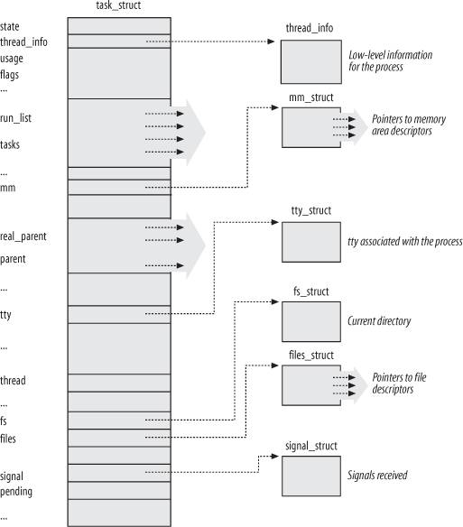 Figure 3-1. The Linux Process Descriptor
Process State
This field describes the state of the process - running, stopped etc. The
current implementation defines it as an array of flags (bits), each describes a
possible state. All states are mutually exclusive, hence at any given time, only
one flag is set and others are all cleared. Possible states
(source):
TASK_RUNNING. The process is either running on a CPU or waiting to be
executed.TASK_INTERRUPTIBLE. The process is suspended (sleeping) until some
condition is met - an hardware interrupt (e.g., disk controller), a lock is
released, a signal is received, etc.TASK_UNINTERRUPTIBLE. Similar to above, except that delivering a signal to
the sleeping process leaves its state unchanged. That is, it can be waken up
only when if certain condition is met, say, a hardware interrupt.TASK_STOPPED. Process execution has been stopped; upon receiving
SIGSTOP, SIGTSTP, SIGTTIN or SIGTTOU.TASK_TRACED. Process execution has been stopped by a debugger - think
ptrace.
Apart from these five states, the state field (and the exit_state field) can
have two additional states. As their name suggests, a process can reach on of
these states only when they are terminated:
EXIT_ZOMBIE. Process is terminated, but its parent hasn’t called wait4()
or waitpid() yet. This state is important because the kernel cannot
discard a process’s descriptor until its parent has called a wait()-like
syscall as per a Unit design principle. This will be detailed later in this
chapter.EXIT_DEAD. The final state: the process is being removed from the system
because its parent has called wait4() or waitpid() for it. The next
phase of the process’ life is the descriptor being deleted. So you may ask, “why
not just delete the descriptor already?”. Well, having this last state is useful
to avoid race conditions due to other threads that execute wait()-like calls
on the same process (see Chapter 5).
The value of the state field is usually set with a simple assignment, e.g.:
The kernel also uses the set_task_state and set_current_state macros to set
the state of a specified process or the current running process. These macros
also ensure atomicity of these instructions. See Chapter 5 for more details on
this.
Identifying a Process
Process descriptor pointers. Each execution context that can be scheduled
independently must have its own process descriptor; even lightweight processes
(threads) have their own task_struct. The strict one-to-one mapping between
processes and process descriptors makes the address of the task_struct
structure a useful means for the kernel to identify processes. These addresses
are referred to as process descriptor pointers.
PIDs. On the other hand, users like to address a process by an integer
called the Process ID or PID. To satisfy this requirement the kernel stores
PID in the pid field of the task_struct. PIDs are numbered sequentially and
there is an upper limit (determined by /proc/sys/kernel/pid_max). When the
kernel reaches this limit, it must start recycling the lower, unused PIDs. If
the rate of process/thread creation exceeds the rate of PID recycle, process
creation is going to fail with likely an EAGAIN (-11) error. The default for
/proc/sys/kernel/pid_max is usually 32K, and can be lifted up to 4,194,303 on
a 64-bit system.
pidmap_array. When recycling PID numbers, the kernel needs to know which of
the 32K numbers are currently assigned and which are unused. It uses a bit map
for that, called the pidmap_array. On 32-bit systems, a page contains 32K bits
(4K bytes), which is perfect for storage of a pidmap_array. On 64-bit systems,
multiple pages might be needed for the pidmap_array depending on the value of
/proc/sys/kernel/pid_max. These pages are never released.
Threads. Each lightweight process has its own PID. To satisfy the user
application requirement that multi-threaded applications should have only one
PID, the kernel groups lightweight processes that belong to the same application
(thread group), and makes system calls like getpid() return the PID of the
thread group leader. In each LWP’s task_struct, the tgid field stores the
PID of the thread group leader and for the thread group leader itself, that
value is equal to its pid value.
PID to process descriptor pointer. Many system calls like kill() use PID
to denote the affected process. It is thus important to make the process
descriptor lookup efficient. As we will see soon enough, Linux has a few tricks
to do that.
Relationships Among Processes
30 Apr 2018
Note: The subtitles in this chapter are reorganized for the ease of my own
understanding. I find them more logically ordered this way than they are in the
book.
Memory Addresses
This chapter focuses on the Intel 80x86 microprocessor memory addressing
techniques, but they should generally apply to most other processors too.
At the highest level, you have a great amount of memory cells that can be used
to store instructions to be executed by the CPU and data to be read by the CPU.
You need to tell the CPU how to access the contents of each cell so you give
them “addresses”, just like every house in America has an address so mails can
be delivered. Each memory address typically points to a single byte in memory.
Segmentation
Intel thinks it is a good idea to split a big program into small logical
segments, each to store partial information about the program. For example,
there can be a code segment for compiled instructions of the program, while
all global and static variables may reside a separate segment called the data
segment. Similarly, there can be stack segment designated for a process’
stack at runtime. This, when applied to the address space of a running process,
splits the entire memory into multiple segments too, each consists of a chunk of
addresses.
Segment Selector
With segmentation, to address a memory location, a pair of identifiers are used:
(Segmentation Selector, Offset). Segmentation Selector is a 16-bit number that
identifies which of the many segments this address lies in, and “Offset” tells
the distance from the start of the selected segment.
Segment Descriptor
Other than a base address, to precisely describe a segment, at least its “size”
needs to be known. There are other characteristics of a segment that the kernel
finds useful, such as which privilege level is required to access addresses in
a segment’s range, is the segment for data or code, etc. These details together,
are stored in a data structure called the Segmentation Descriptor.
Global Descriptor Table (GDT) and Local Descriptor Table (LDT)
Now that we have a set of segments, each with its descriptor, we need an array
to store all these descriptors. This array is called a Descriptor Table. There
is usually a Global Descriptor Table or GDT that’s shared by all processes (they
use the same segments for addressing), and optionally a per-process table called
the Local Descriptor Table.
Both tables are stored in memory themselves. To locate them, their addresses are
stored in two registers: gdtr and ldtr, respectively.
Logical Address and Linear Address
In Intel’s design, all addresses used in programs should be “Logical Addresses”,
which are (Segmentation Selector, Offset) pairs. But the CPU doesn’t
understand these pairs, so there is a designated hardware component that
translates logical addresses into Linear Addresses, which are 32-bit
unsigned integers that range from 0x00000000 to 0xffffffff, for a memory of 4
gig bytes. This hardware component is called the Segmentation Unit.
Segmentation Unit
Segmentation unit’s sole purpose is to translate logical addresses into linear
addresses. It takes a (Segment Selector, Offset) pair, from which it gets the
index into the Descriptor Table (array) of the segment to select, which then
gives the starting (base) address of that segment. Then by multiplying Offset by
8 (each descriptor in the Descriptor Table is 8-byte long) and adding the
product to the base, it gets a linear address.
Fast Address Translation
As you can see from above section, each address translation involves one read of
the Descriptor Table (to get the descriptor of the selected segment), which sits
in memory. Because the descriptor of a segment rarely changes, it’s possible to
speed up translations by loading the descriptor (8 byte) into a dedicated
register, so subsequent translations don’t need to read memory, which is a
magnitude slower than reading a register.
Segmentation in Linux
Though the concept of segmentation and splitting programs into logically related
chunks is kind of enforced by Intel processors, Linux doesn’t use segmentation
much. In fact, it defines barely a handful of segments even though the maximum
allowed number is 2^13 (13-bit used for index in Segment Selector).
Four main segments Linux uses are: Kernel Code Segment, Kernel Data Segment,
User Code Segment, and User Data Segment. The Segment Selector values of these
are defined by the macros __KERNEL_CS, __KERNEL_DS, __USER_CS and
__USER_DS. To address the kernel code segment, for example, the kernel simply
loads the value defined by __KERNEL_CS into the segmentation register.
The descriptors of each segment are as follows:
| Segment |
Base |
G |
Limit |
S |
Type |
DPL |
D/B |
P |
| user code |
0x00000000 |
1 |
0xffff |
1 |
10 |
3 |
1 |
1 |
| user data |
0x00000000 |
1 |
0xffff |
1 |
2 |
3 |
1 |
1 |
| kernel code |
0x00000000 |
1 |
0xffff |
1 |
10 |
0 |
1 |
1 |
| kernel data |
0x00000000 |
1 |
0xffff |
1 |
2 |
0 |
1 |
1 |
As you can see all four segments start at address 0. This is not a mistake. In
Linux, a logical address always coincides with a linear address. Again, Linux is
not a big fan of segmentation and spends more of its design in an alternative
paging mechanism - paging - which we will talk about next.
The Linux GDT
As mentioned above, the GDT is an array of Segment Descriptor structs. In Linux,
the array is defined as cpu_gdt_table, while the address and size of it are
defined in the cpu_gdt_descr array. It is an array because there can be
multiple GDTs: on multi-processor systems each CPU has a GDT. These values are
used to initialize the gdtr register.
Both arrays are 32-element long, which include 18 valid segment descriptors,
and 14 null, unused or reserved entries. Unused entries are there so that
segment descriptors accessed together are kept in the 32-byte hardware cache
line.
The Linux LDTs
These are similar to GDTs and are not commonly used by Linux applications except
for those that run Windows applications, e.g., Wine.
Paging in Hardware
Just as the segmentation unit translates logical addresses into linear
addresses, another hardware unit, the paging unit, translates linear addresses
into physical addresses.
Page, Page Frame and Page Table
For efficiency, linear addresses are grouped into fixed-length chunks called
pages. Contiguous linear addresses are mapped into contiguous physical
addresses. Each of these groups is called a physical page frame. Note that
while pages are blocks of data, page frames are physical constitute of the main
memory.
The data structure that maps pages to page frames is called page table.
Regular Paging
The word “regular” is relative to the extended or more advanced paging
techniques that are required for special cases that we will cover later in this
chapter. This section is about the fundamental idea of how paging is done in
Intel hardware.
As previously mentioned, the paging unit translates pages as the smallest unit
and not individual addresses. The default page size on Linux is 4KB (2^12
bytes). So the 20 most significant bits of a 32-bit address alone can uniquely
identify a page (the last 12 bits will be within a page). An rudimentary idea of
implementing paging would be to have a table of (linear page, physical page)
tuples, and try to match the 20 most significant bits of a linear address in the
table. However, that implies that we would need 2^20 entries in the array, or at
least reserve space for that many entries if the implementation is a linear
array, even when the process doesn’t use all addresses in the range. With each
entry taking up 4 bytes (32 bits), our table would take 4MB of memory. Of course
there is room for improvement.
The idea is to split the 20 most significant bits into two 10-bit segments; the
first 10 to be used as index to a higher level Page Directory whose entries are
physical addresses to secondary Page Tables, and the rest 10 bits as index to a
particular Page Table. With demand paging (page frames are only assigned when
actually requested), the secondary Page Tables are added as the process requests
more memory. In the extreme case that the process uses all 4GB address space,
the total RAM used for the Page Directory and all Page Tables will be 4MB, no
more than the basic algorithm above.
This is called 2-level paging and you will see the idea getting generalized into
multi-level paging on systems with bigger address spaces, e.g., 64 bit systems.
The physical address of the Page Directory is stored in cr3. From there the
paging unit gets the physical address to a Page Table, and in turn it gets the
physical address of a page frame a page is mapped into. Then by adding the least
significant 12 bits of a linear address (Offset), it gets a 32 bit physical
address.
Page Directory/Table Data Structure
In Linux, it is a 32-bit compound integer of the following bits:
Present flag. If set, the referred-to page or page table is in main memory. If
not, the linear address requested is saved to cr2 and exception 14 (Page
Fault) is generated. The kernel relies on page faults to assign additional page
frames to a process.
20 most significant bits of a page frame physical address. Because of the 4KB
page size, the last 12 bits of a physical address doesn’t matter.
Accessed flag. Whether or not the referred-to page or page table is accessed.
This flag may be used to decide which pages to swap out in case the system is
running low on memory.
Dirty flag. Whether or not the referred-to page or page table is written to.
Similar use as the accessed flag.
Read/Write flag. Access right of the page frame or page table: read-only or
writable.
User/Supervisor flag. Privilege needed to access the page or page table: user
process or kernel.
PCD and PWT flags. Controls some hardware cache behaviors. Explained below at
“Hardware Cache”.
Page Size flag. Controls the page size, if not 4KB. See “Extended Paging” for
details.
Global flag. Controls TLB flush behaviors.
Extended Paging
On newer 80x86 processors, larger pages are supported (4MB instead of 4KB) and
thus more bits are needed for the Offset part and fewer for Page Directory and
Page Table. In fact, since the Offset takes 22 bits, the 10 most significant
bits all be used as an index into the Page Directory, thus eliminating the need
for secondary Page Tables.
Hardware Protection Scheme
Different from the segmentation unit, which allow multiple privilege levels (0,
1, 2, 3), the paging unit only allows two: User/Supervisor. Furthermore, only
two rights are associated with pages: Read/Write.
Physical Address Extension (PAE) Paging Mechanism
The amount of RAM supported by a processor is limited by the number of address
pins connected to the address bus. As the servers grow, Intel extended the
address pins of their 80x86 processors from 32 to 36. This makes them able to
address up to 2^36 = 64GB memory. Adapting to this change, Linux tweaked the
number of bits used to index Page Directory, Page Table and as Offset, and in
some cases, added an additional table before Page Directory - Page Directory
Pointer Table. But the same general idea applies.
Paging for 64-bit Architectures
On 64-bi systems, there are 64 address pins. It certainly doesn’t make sense to
use all 64-12 = 52 most significant bits (assuming a usual page size of 4KB) as
that would give a maximum of 256TB address space! So fewer bits are used, and
multi-level paging is used. The actual split of bits varies from architecture to
architecture.
Hardware Cache
Typical RAMs access time is in the order of hundreds of clock cycles. That is a
LOT of time comparing to instruction executions. To remedy the huge speed
mismatch between the CPU and the memory, fast hardware cache memories are
introduced. Based on locality principle, data recently fetched from memory, or
those next to them, are kept in the cache. And over the years, multiple levels
of cache are added, each with different speed and cost characteristics.
A new unit was introduced along with the hardware cache: line. It refers to
a certain block of contiguous data in memory or in cache. Data are always read
into cache or cleared in multiple of line. A line is usually several dozens of
bytes.
On multi-processor systems, each CPU has its own hardware cache. The
synchronization between two caches is important, and usually is done by a
dedicated hardware unit so the OS doesn’t have to care. But one interesting
feature of some cache is that the hardware allows the cache sync policy
(Write-Through v.s. Write-Back) to be selected and set by the OS. In Linux,
Write-Back is always selected.
Translation Lookaside Buffers (TLB)
Besides general purpose cache, 80x86 processors include another cache called the
Translation Lookaside Buffer (TLB), to speed up linear address translation.
When a linear address is used for the first time, the corresponding physical
address is computed through page table lookups, and stored in the TLB for future
reference. Note that because each process has its own page tables, the TLB is
flushed during a context switch.
On multi-processor systems, each CPU has its own TLB. Unlike hardware cache, two
TLBs don’t need to be synchronized because they are being used by two processes
that have different page tables any way.
Paging in Linux
Linux adopts a common paging model that fits both 32-bit and 64-bit
architectures. A four-level paging model is used, and consists of the following:
- Page Global Directory
- Page Upper Directory
- Page Middle Directory
- Page Table
For 32-bit architectures, two paging levels are sufficient so the Page Upper
Directory and Page Middle Directory are eliminated - by saying that they contain
zero bits.
Linux’s handling of processes relies heavily on paging. The automatic linear to
physical address translation makes a few design objectives feasible:
- Assign a different physical address space to each process, ensuring
isolation.
- Distinguish pages from page frames. This allows the same page to be written
to a page frame, or swapped to disk, and then read back into memory at a
different page frame.
Process Switch. The essence of process switch is saving the value of cr3
into the old process’ descriptor, and loading the new process’ Page Global
Directory physical address into cr3.
The Linear Address Fields
This and the following section (Page Table Handling) detail a few important
macros and functions related to the Page Table data structures. I did not read
them line by line and thus don’t have a lot to note down. I can always come back
to them when needed.
Page Table Handling
Ditto.
Physical Memory Layout
This is the fun part about memory management. To start managing memory, the
kernel first needs to know where all the memory chunks are, and how big each is.
Note that not all physical memory is usable by the kernel. Some of them may be
reserved by the BIOS, some reserved for IO device memory mapping, for example.
In general, the kernel considers the following reserved (that cannot be
dynamically assigned or swapped to disk):
- Those falling in the “unavailable” physical address ranges
- Those containing the kernel’s own code and data
Kernel address. In general, the Linux kernel is installed in RAM starting
from the physical address 0x00100000 - i.e., from the second megabyte. The total
number of page frames required depends on the configuration, but typically a
Linux kernel image can fit in 3MB of memory.
Why is the kernel not loaded to the first megabyte?:
- Page frame 0 is used by BIOS to store system hardware configurations during
its Power-On Self-Test (POST).
- Physical address 0x000a0000 to 0x000fffff are usually reserved for BIOS
routines amd to map internal memory of ISA grapic cards.
- Additional frames within the first megabyte may be reserved by specific
computer models.
During boot, the kernel queries BIOS to learn the size of the physical memory,
and the list of physical address ranges. It does this in the
machine_specific_memory_setup() function. Right after this, in the
setup_memory() function, it establishes the following variables:
| Variable name |
Description |
| num_phypages |
Page frame number of the highest usable page frame |
TODO: Fill the table.
Figure 2-13 shows how the first 3MB of RAM are filled by Linux.
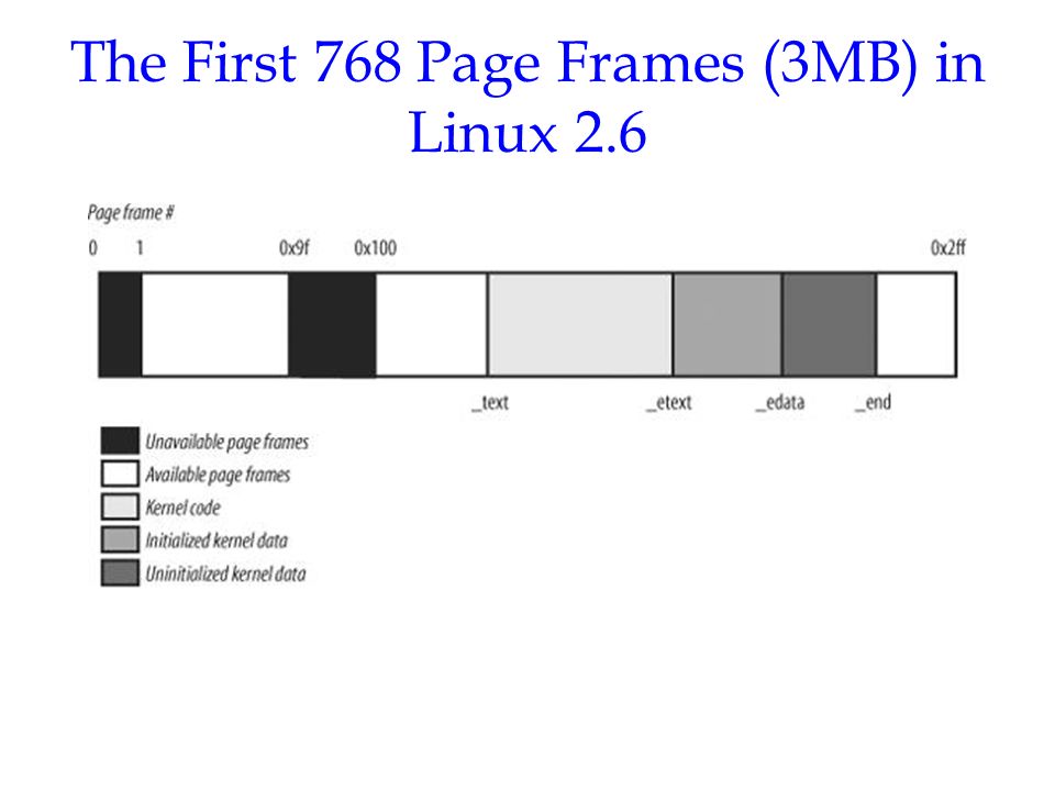
Starting at the physical address 0x00100000 is the symbol _text, which is the
address of the first byte of kernel code. Following it there are _etext,
_edata, and _end. They denote: end of text, end of data, and end of kernel.
Between _etext and e_data is the initialized data structures, and the next
is uninitialized data.
Process Page Tables
A process’ linear address space is divided into two parts:
- User or kernel mode: 0x00000000 to 0xbfffffff
- Kernel mode only: 0xc0000000 to 0xffffffff
I.e., the lowest 896MB are pages used for kernel code and data.
Every process has a different Page Global Directory with different entries, but
all of them share the entries for the lowest 896MB of linear address space -
kernel.
Kernel Page Tables
The kernel maintains a set of page tables of its own, rooted at a master kernel
Page Global Director. After system initialization, this set of page tables is
never directly used by any process or kernel thread.
Chapter 8 will explain how the kernel ensures changes to the master kernel Page
Global Directory always reflect in each process’ Page Global Directory. This
chapter will next explain how the kernel initializes its own page tables. It
is a two-phase activity, and note that right after when kernel is loaded
into memory, the CPU is running in real mode, with paging disabled.
In the first phase the kernel creates a limited address space including kernel’s
code and data segments, the initial Page Tables, and 128KB for some dynamic data
structures.
In the second phase, the kernel sets up Page Tables for all of the existing RAM.
Provisional kernel Page Tables
A provisional Page Global Directory is initialized during kernel compilation
time, while provisional Page Tables are initialized at runtime, by the
startup_32() assembly function defined in arch/i386/kernel/head.S.
The provisional Page Global Directory is contained in the swapper_pg_dir
variable. Again, this is computed at compile time and is known at run time. The
provisional Page Tables are stored starting from pg0, right after _end in
the kernel image. For simplicity, we will assume the kernel image, the
provisional Page Tables, plus the 128KB dynamic space can fit into the first 8MB
of RAM. In order to map 8MB of RAM, two Page Tables are required (??).
The objective here is to allow these 8MB of RAM to be addressed in both real
mode and in protected mode. Therefore, a mapping from both the linear
addresses 0x00000000 through 0x007fffff (first 8MB in real mode) and the linear
addresses 0xc0000000 through 0xc07fffff (first 8GB in protected mode) is needed.
In other words, the kernel during initialization can address the first 8MB of
RAM by either linear addresses identical to the physical ones, or 8MB worth of
linear addresses, starting from 0xc0000000.
Identity Mapping. The mapping of linear addresses 0x00000000 through
0x007fffff to the same physical addresses is usually referred to as Identity
Mapping. It is important because most CPUs are pipelined; that is, multiple
instructions spit by the CPU might be in action in multiple stages. As soon as
the MMU/paging unit is turned on, some old instructions spit by CPU with
physical addresses may be in flight. For them to work, the first 8MB RAM range
needs to be mapped too. StackOverflow
answer.
The kernel creates that mapping by filling all the swapper_pg_dir (the
provisional Page Global Directory) entries with zeroes, except for entries 0, 1,
0x300 and 0x301; the latter two entries span all linear addresses between
0xc0000000 and 0xc07fffff:
The address field of entries 0 and 0x300 is set to the physical address of
pg0 (the byte immediately following the _end symbol), while the address
field of entries 1 and 0x301 is set to the physical address of the page frame
following pg0. Again, two page tables are needed to map 8MB of RAM.
Final kernel Page Table when RAM size is less than 896MB
The final kernel Page Tables should map linear addresses from 0xc0000000 through
0xffffffff to physical addresses starting at 0x0.
Final kernel Page Table when RAM size is between 896MB and 4096MB
Final kernel Page Table when RAM size is more than 4096MB
Handling the Hardware Cache and the TLB
Handling the hardware cache
As mentioned earlier, hardware caches are addressed by cache lines. The
L1_CACHE_BYTES defines the size of the cache line. To optimize for cache
hit rate, the kernel does the following tricks when dealing with data
structures:
- Most frequently used fields are placed at the lower offset within a data
structure, so that they can be cached in the same line. Compare this to
ording fields alphabetically or in groups of types.
- When allocating a large set of data structures, the kernel tries to store
each of them in memory in such a way that all cache lines are used
uniformly.
Cache synchronization. As mentioned earlier, on 80x86 microprocessors
hardware cache synchronization (between CPUs) are taken care of by the hardware
and is transparent to the kernel.
Handling the TLB
Contrary to that, TLB flushes have to be done by the kernel because it is the
kernel that decides when a mapping between a linear address and a physical
address is no longer valid.
TLB synchronization between CPUs are done by the means of a Interprocessor
Interrupts. That is, a CPU that is invalidating its TLB sends a signal to
others to force them to do a flush as well.
Generally speaking, a process switch indicates a TLB flush. However there are a
few exceptional cases in which a TLB flush is not necessary:
- When the switch is to another process that uses the same set of page tables
as the process being switched from.
- When performing a switch between a user process and a kernel thread. That is
because kernel threads do not have their own page tables; rather, they use
the set of page tables owned by the user process that was scheduled last for
execution on the CPU.
Lazy TLB flushes. We mentioned earlier that TLB synchronization is done
through one CPU sending an Interprocessor Interrupt to others. When a CPU that
is running a kernel thread gets such an interrupt, it simply ignores it and
skips the requested TLB flush as kernel threads don’t access user processes’
address space (the lower 3GiB) - they won’t reference the TLB entries any way.
This is called the lazy TLB mode. However, the kernel remembers that an
interrupt has been received so when it switches back to a user process, it
correctly issues the TLB flush.
29 Apr 2018
Definition
Mine, yours, his, hers, theirs. Note the distinction between a possessive
pronoun and a possessive adjective (e.g., my, your, his, her, their).
Gender and Number
Possessive pronouns have to agree with both the gender and number of the
object owned or possessed, and not the owner. For example, “The girls read the
books of theirs” - Las muchachas leen los libros suyos. Full table:
| Singular |
Plural |
| mío, míos mine |
nuestro, nuestros ours |
| mía, mías mine |
nuestra, nuestras ours |
| tuyo, tuyos, yours |
vuestro, vuestros yours |
| tuya, tuyas, yours |
vuestra, vuestras yours |
| suyo, suyos, his, hers, theirs, (formal) yours |
suyo, suyos, theirs, (formal) yours |
| suya, suyas, his, hers, theirs, (formal) yours |
suya, suyas, theirs, (formal) yours |
In contrast, these are the possessive adjectives. You may have noticed that the
first and second person informal plural have the same form as adjective as well
as pronoun.
| Singular |
Plural |
| mi, mis my |
nuestro, nuestros our |
| |
nuestra, nuestras our |
| tu, tus your |
vuestro, vuestros your |
| |
vuestra, vuestras your |
| su, sus his, her, (formal) your |
su, sus their, your |
Possessive Pronouns Following ser
It is the same form as in English. For example, “This book is mine” - Este
libro es mío, “This table is yours” - Esta mesa es tuya.
Possessive Pronouns Expressing “of mine/yours/his/her/ours/theirs”
In English we like to say “a friend of mine” or “an adventure of yours”. In
Spanish, there is no need to insert a de between the object owned and the
possessive pronoun. To say “a friend of mine” it is simply un amigo mío.
Possessive Pronouns in Comparisons
When two things are compared against each other, there are two forms that can be
used. The first is the “regular comparison” that ranks the two subjects, i.e.,
“A is better/worse/taller/shorter than B”. In the second form, two subjects are
brought up together but no explicit ranking is drawn. For example, “this house
is mine, while that one is yours”, or “I like my house, as well as yours”.
Regular Comparisons
| more … than |
más ... que |
| less … than |
menos ... que |
| as … as |
tan ... como |
Examples:
| My friend is taller than yours |
Mi amigo es más alto que el tuyo |
| Their house is less elegant than yours |
Su casa es menos elegante que la tuya |
Irregular Comparatives
Unlike English, there are only four irregular comparatives in Spanish. They
are:
mejor, mejores    better        mayor, mayores      older
peor, peores      worse         menor, menores      younger
When used with these comparatives, possessive pronouns follow the same rules
above.
Comparative Statements
In the second form of comparison possessive pronouns follow the same rules as
well. For example:
| Their house is dirty but ours is clean |
Su casa está sucia pero la nuestra está limpia |
| Her books are in the kitchen and mine are in the dinning room |
Su libros están en la cocina y las míos están en el comedor |
29 Apr 2018
Definition
When the noun after a number is omitted, the number serves as a pronoun. For
example, “How many books do you have?”, “I have three (kids)”. Or, “Which book
is your favorite?”, “The third (book)”.
Both cardinal and ordinal numbers can be used as pronouns.
Numbers Below 10
| Cardinal Numbers |
Ordinal Numbers |
| uno, una |
primero, primera |
| dos |
segundo, segunda |
| tres |
tercero, tercera |
| cuatro |
cuarto, cuarta |
| cinco |
quinto, quinta |
| seis |
sexto, sexta |
| siete |
séptimo, séptima |
| ocho |
octavo, octava |
| nueve |
noveno, novena |
| diez |
décimo, décima |
Notes:
- Ordinal numbers take gender.
- When referring to a masculine noun, “first” and “third” drop the trailing
o and become primer and tercer, respectively.
Numbers Above 10
Cardinal numbers are the same weather below or above 10, but ordinal numbers can
be seen in two ways:
- “number-
avo”, e.g., onceavo (11th), doceavo (12th) and treceavo (13th)
- but more commonly, “
el number”, e.g., el doce (11th), el doce (12th)
and el trece (13th)
Cardinal Numbers as Pronouns
Pretty much the same as in English. For example, ¿Cuántos libros tienes?,
Tengo tres..
Ordinal Numbers as Pronouns
The only additional thing needs to be noted is that ordinal numbers have to
agree on gender with the omitted noun. For example, El árbol es el séptimo
(the tree is the seventh) and La lámpara es la segunda (the lamp is the
second). Note that the definitive articles used need to agree on gender too.